OVarFlow 2
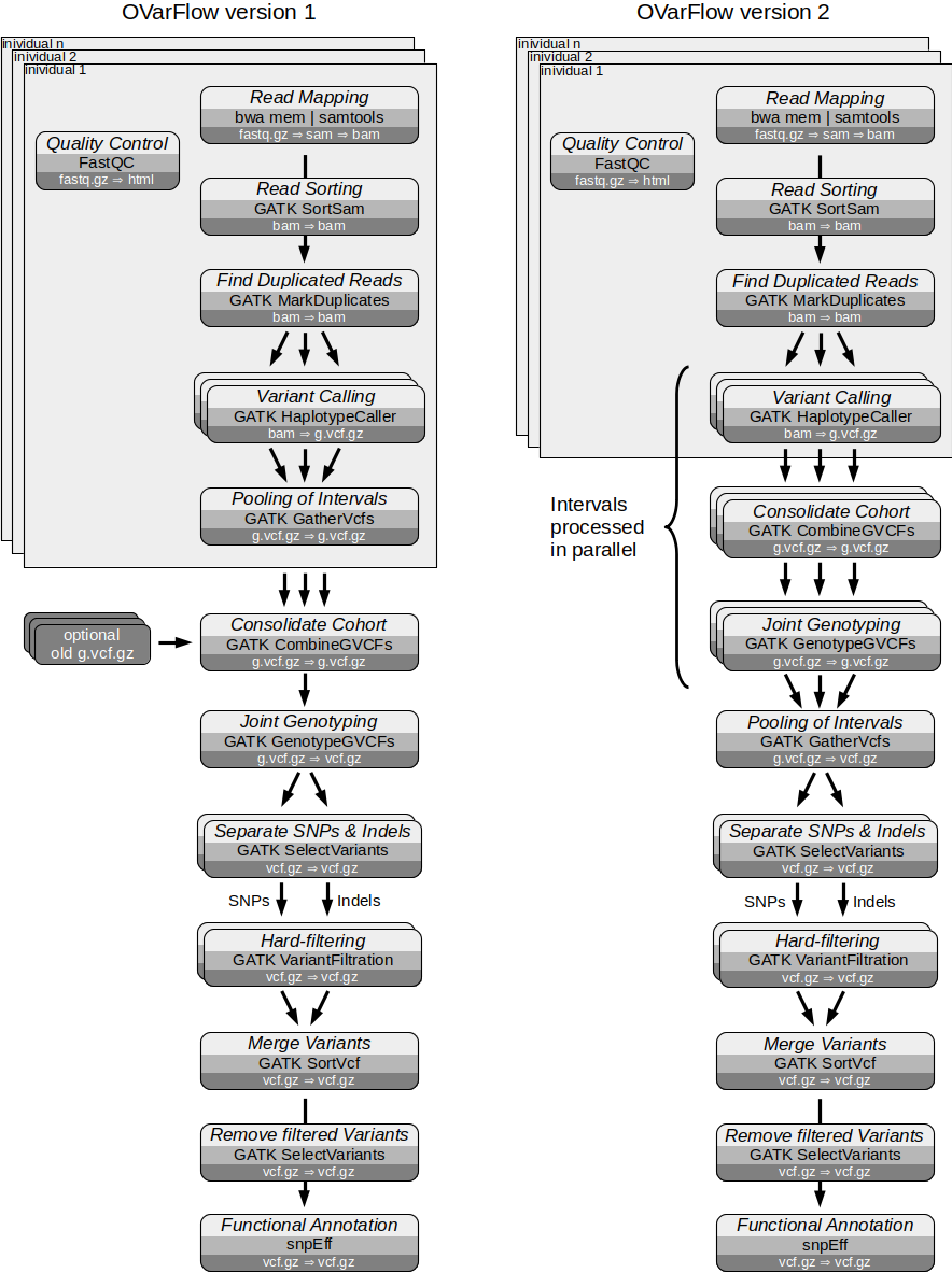
When processing large cohorts of individuals (more than 50 to 100 individuals), OVarFlow 1 offered some additional leeway for performance improvements. These issues were addressed in OVarFlow 2. Previously, only the HaplotypeCaller was parallelized based on genomic intervals that could be processed simultaneously. By rearranging two steps of the workflow, the GATK tools CombineGVCFs and GenotypeGVCFs are able to process the same genomic intervals that the HaplotypeCaller was utilizing. This allows these two steps, which can take quite a long time for large cohorts, to be dramatically accelerated through parallelization.
However, the first version of OVarFlow remains a valid tool for analyzing small to medium sized cohorts. OVarFlow 2 will be especially beneficial when analyzing very large cohorts, comprising hundreds of individuals. For instance, when using whole genome sequencing data for genome-wide association studies (GWAS), OVarFlow 2 provides significant improvements which can be in the order of several weeks when dealing with very large cohort sizes.
Usage of OVarFlow 2
Fortunately, OVarFlow 2 could be designed in a way that the usage remains identical to the first generation of the workflow. This also includes the CSV and Yaml configuration files. Therefore, all previous usage descriptions remain valid.
Only one alteration on the end user side has to be considered: preexisting GVCF files (*.g.vcf.gz) cannot be included in the analysis. To remain fully compatible with OVarFlow 1, the corresponding entry was not remove from the CSV configuration file. If any GVCF files are specified here, OVarFlow 2 will war the user, that these files won’t be used in the analysis. Instead, the fastq files should be provided for all individuals to be analyzed.
The only real difference when executing OVarFlow 2 is that a different Snakefile has to be specified on the command line, namely Snakefile_OVarFlow2. Nevertheless, a brief recap of the most important commands shall be given here:
Perform a dry run of the workflow:
snakemake -np --cores <threads> --snakefile Snakefile_OVarFlow2
Perform the actual run:
snakemake -p --cores <threads> --snakefile Snakefile_OVarFlow2
Overview of the workflow
Here, a brief overview of the tools used in the workflow and the sequence of their use is given. The tools used are identical to the first version of OVarFlow, but due to some rearrangements a higher degree of parallelization was achieved.
Data pre-processing
fastqc: quality control of reads (optional but recommended)bwa mem: mapping to the reference genomegatk SortSam: sorting of the readsgatk MarkDuplicates: as the name implies
Preparation of variants
gatk HaplotypeCaller: actual variant calling (on intervals)gatk CombineGVCFs: pooling of called individuals (on intervals)gatk GenotypeGVCFs: genotyping of the called variants (on intervals)gatk GatherVcfs: pooling of intervalsgatk SelectVariants: separating of SNPs and indelsgatk VariantFiltration: hard filtering of SNPs and indelsgatk SortVcf: merging of SNPs and indelsgatk SelectVariants: removal of filtered variants
Variant annotation
snpEff: variant annotation
Compared to OVarFlow 1, only the steps 5, 6 and 7 are rearranged and use some slightly modified commands (apart from some changes to the Snakefile that were necessary to make things work). Here, the most basic syntax of these three commands shall be provided, but no special Java options or tuning parameters will be given.
Pooling of intervals per individual
1gatk CombineGVCFs -O <interval_n.g.vcf.gz> -L <interval_n.list> -R <reference_genome> \↵
2 -V <individual_1/interval_n.g.vcf.gz> -V <individual_2/interval_n.vcf.gz> \↵
3 ... -V <individual_n/interval_n.g.vcf.gz>
Processing the Genotypes
1gatk GenotypeGVCFs -L <interval_n.list> -R <reference_genome> \↵
2 -V <interval_n.g.vcf.gz> -O <interval_n.g.vcf.gz>
Gathering of the intervals
1gatk GatherVcfs -o <all_genotyped_calls.g.vcf.gz> -I <interval_1.g.vcf.gz> -\↵
2 -I <interval_2.vcf.gz> ... -I <interval_n.g.vcf.gz
Comparison of OVarFlow 1 & 2
The flow chat below illustrates the differences in the workflow between version one and two. The most obvious is that GATK CombinegVCFs and GenotypeGVCFs will also work in parallel. This was achieved by postponing Pooling of the Intervals.
Comparative Benchmarking
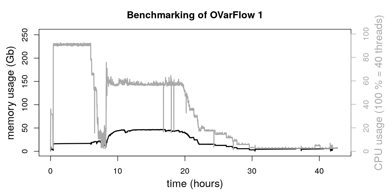
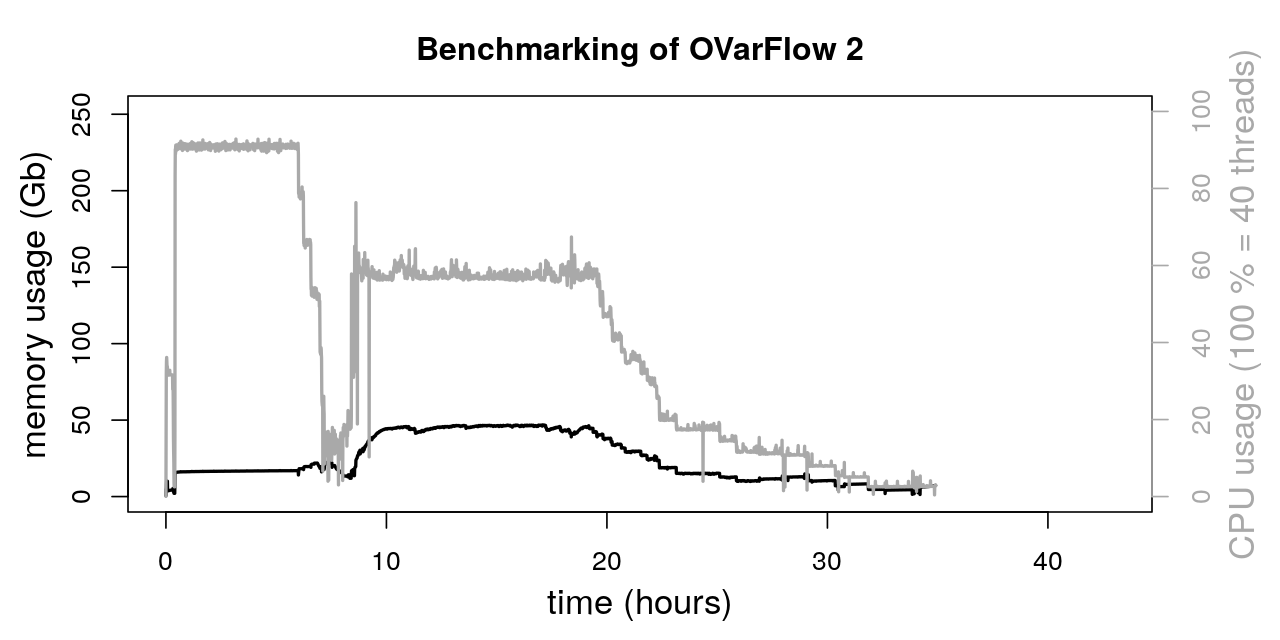
As explained before, OVarFlow 2 advances parallelizition by performing more computations on genomic intervals. To see the impact of parallelizing GATK CombineGVCFs and GenotypeGVCFs, the entire workflows of OVarFlow 1 and 2 were benchmarked. Benchmarking was performed as previously described in section “Resource Optimization -> Benchmarking & Optimizations -> Entire Workflow”. In addition, the same sequencing data and hardware resources were used as before.
Reference organism |
Gallus gallus |
Reference genome |
GCF_000002315.6 (GRCg6a) |
Sequencing data |
ERR1303580, ERR1303581, ERR1303584, ERR1303585, ERR1303586, RR1303587 |
Both workflows utilized the same yaml configuration file:
 1heapSize:
 2    SortSam         : 10
 3    MarkDuplicates  : 2
 4    HaplotypeCaller : 2
 5    GatherIntervals : 2
 6    GATKdefault     : 12
 7
 8ParallelGCThreads:
 9    SortSam         : 2
10    MarkDuplicates  : 2
11    HaplotypeCaller : 2
12    GatherVcfs      : 2
13    CombineGVCFs    : 2
14    GATKdefault     : 4
15
16Miscellaneous:
17    BwaThreads      : 6
18    BwaGbMemory     : 4
19    GatkHCintervals : 4
20    HCnpHMMthreads  : 4
21    GATKtmpDir      : "./GATK_tmp_dir/"
22    MaxFileHandles  : 300
23    MemoryOverhead  : 1
24
25Debugging:
26    CSV             : False
27    YAML            : False
The actual computations were performed on a single cluster node (SGE) reserved exclusively for OVarFlow. The cluster node provided 20 cores / 40 threads (Intel Xeon E5-2670) and 251.9 Gb of main memory.
The total runtime of both workflows was:
OVarFlow 1: 42.675 h
OVarFlow 2: 34.91 h
Thereby, the total runtime of OVarFlow 2 could be reduced by about 22 % compared to OVarFlow 1. Of course, this value is very specific for the given hardware, sequencing data, reference genome, and settings mentioned above. By utilizing even more intervals in parallel, further runtime reduction might be possible. However, a time saving of 20 % by utilizing OVarFlow 2 is a reasonable estimate.